Contextualized Bayesian Networks#
For more details, please see the NOTMAD preprint.
import numpy as np
import matplotlib.pyplot as plt
%matplotlib inline
from contextualized.dags.graph_utils import simulate_linear_sem

n = 1000
C = np.linspace(1, 2, n).reshape((n, 1))
W = np.zeros((4, 4, n, 1))
W[0, 1] = C - 2
W[2, 1] = C**2
W[3, 1] = C**3
W[3, 2] = C
W = np.squeeze(W)
W = np.transpose(W, (2, 0, 1))
X = np.zeros((n, 4))
for i, w in enumerate(W):
    x = simulate_linear_sem(w, 1, "uniform", noise_scale=0.1)[0]
    X[i] = x
%%capture
from contextualized.easy import ContextualizedBayesianNetworks

cbn = ContextualizedBayesianNetworks(
    encoder_type='mlp', num_archetypes=16,
    n_bootstraps=2, archetype_dag_loss_type="DAGMA", archetype_alpha=0.,
    sample_specific_dag_loss_type="DAGMA", sample_specific_alpha=1e-1,
    learning_rate=1e-3)
cbn.fit(C, X, max_epochs=10)
GPU available: True (mps), used: False
TPU available: False, using: 0 TPU cores
IPU available: False, using: 0 IPUs
HPU available: False, using: 0 HPUs

  | Name      | Type      | Params
----------------------------------------
0 | encoder   | MLP       | 1.8 K
1 | explainer | Explainer | 256
----------------------------------------
2.0 K     Trainable params
0         Non-trainable params
2.0 K     Total params
0.008     Total estimated model params size (MB)
# We can measure Mean-Squared Error to measure likelihood of X under predicted networks.
mses = cbn.measure_mses(C, X)
print(np.mean(mses))
/opt/homebrew/lib/python3.10/site-packages/pytorch_lightning/trainer/connectors/data_connector.py:430: PossibleUserWarning: The dataloader, predict_dataloader, does not have many workers which may be a bottleneck. Consider increasing the value of the `num_workers` argument` (try 10 which is the number of cpus on this machine) in the `DataLoader` init to improve performance.
  rank_zero_warn(
1.77282994611765
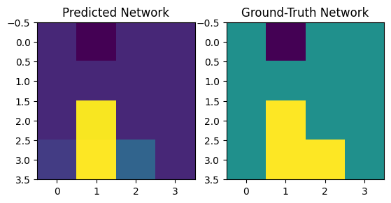
# Predict and visualize network
predicted_networks = cbn.predict_networks(C)

f, axarr = plt.subplots(1, 2)
axarr[0].imshow(predicted_networks[0])
axarr[1].imshow(W[0])
axarr[0].set_title("Predicted Network")
axarr[1].set_title("Ground-Truth Network")
Text(0.5, 1.0, 'Ground-Truth Network')
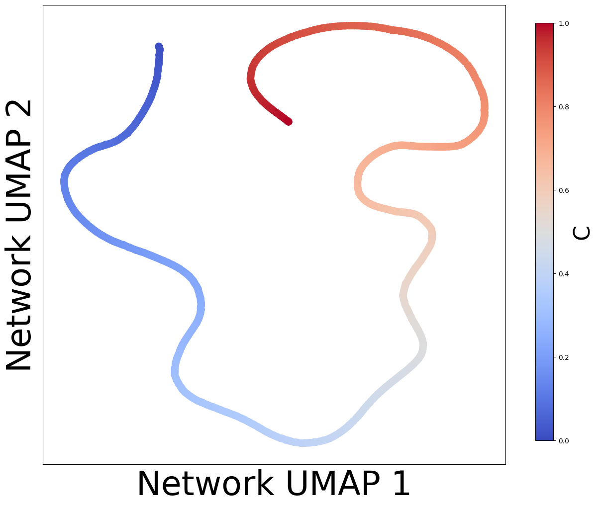
# We can embed networks in lower-dimensional spaces to visualize distributions.
from contextualized.analysis.embeddings import plot_embedding_for_all_covars
import umap
import pandas as pd
low_dim_networks = umap.UMAP().fit_transform(predicted_networks.reshape((n, -1)))
plot_embedding_for_all_covars(low_dim_networks[:, :2], pd.DataFrame(C, columns=['C']),
                             xlabel="Network UMAP 1", ylabel="Network UMAP 2")
# In this case, there is only 1 context variable so the embeddings are not very interesting.
Acyclcity Regularizers#
Contextualized Bayesian Networks are available with two types of DAG losses:
These can be chosen for the archetypes and the sample-specific graphs independently by using the dag.loss_type parameter:
archetype_dag_loss_type="NOTMAD" or archetype_dag_loss_type="DAGMA"
and similarly
sample_specific_dag_loss_type="NOTMAD" or sample_specific_dag_loss_type="DAGMA".
NOTEARS has parameters:
alpha(float)rho(float)use_dynamic_alpha_rho(Boolean)
DAGMA has parameters:
alpha(strength, default 1e0)s(max spectral radius, default 1)
Factor Graphs#
To improve scalability, we can include factor graphs (low-dimensional axes of network variation).
This is controlled by the num_factors parameter. The default value of 0 turns off factor graphs and computes the network in full dimensionality.
We will explore this more deeply in the next notebook.